Can I Get Excel to Recognize a Trend and Continue It
Trend Function in Excel
The TREND function in Excel is a statistical function that computes the linear trend line based on the given linear data set. It calculates the predictive values of Y for given array values of X and uses the least square method based on the given two data series. The TREND function in Excel returns numbers in a linear trend matching known data points. That is, the existing data on which the trend in Excel predicts the values of Y dependent on values of X needs to be linear.
Table of contents
- Trend Function in Excel
- What is the least square method?
- Syntax
- How to Use TREND Function in Excel?
- Example #1
- Example #2 – Predicting the Sales Growth
- Things to Remember
- TREND Function in Excel Video
- Recommended Articles
What is the least square method?
It is a technique used in the regression analysis Regression analysis depicts how dependent variables will change when one or more independent variables change due to factors, and it is used to analyze the relationship between dependent and independent variables. Y = a + bX + E is the formula. read more that finds the line of best fit The line of best fit is a mathematical concept that correlates points scattered across a graph. read more (is a line through a scatter graph of data points that foremost indicates the relationship between those points) for a given dataset, which helps to visualize the relationship between the data points.
Syntax
Below is the TREND formula in Excel.
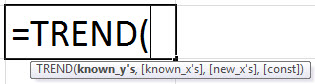
Arguments
For the given linear equation, y = m*x + c
Known_y's: It is a required argument representing the set of y-values we already have as existing data in a dataset that follows the y = mx + c.
Known_x's: It is an optional argument representing a set of x-values that should be of equal length to the set of known_y's. If this argument is omitted, the set of known_x's takes the value (1, 2, 3 … so on).
New_x's: It is also an optional argument. These are the numeric values that represent the new_x's value. If the new_x's argument is omitted, it is set to be equal to the known_x's.
Const: It is an optional argument specifying whether the constant value c equals 0. If const is TRUE or omitted, c is calculated normally. If false, c is taken as 0 (zero), and the values of m are adjusted so that y = mx.
How to Use TREND Function in Excel?
The TREND function in Excel is very simple and easy to use. Let us understand the working of the TREND function by some examples.
You can download this TREND Function Excel Template here – TREND Function Excel Template
Example #1
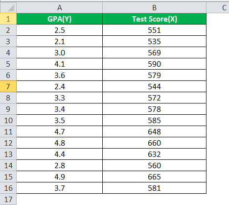
Suppose we have data for test scores with their GPA in this example. Now using this given data, we need to predict the GPA. We have the existing data in columns A and B. The current GPA values corresponding to scores are Y's known values. The existing values of the score are the known values of X. We have given some values for X values as a score, and we need to predict the Y values, that is, the GPA, based on the existing values.
Existing Values:
Given Values and Values of Y to be predicted:
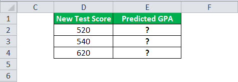
To predict the values of the GPA for given test scores in cells D2, D3, and D4, we will use the TREND function in Excel.
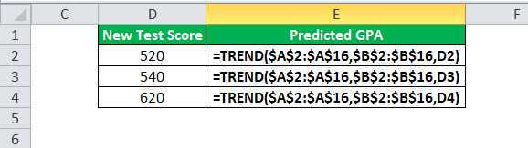
The TREND formula in Excel will take the existing values of known X and Y. We will pass the new values of X to calculate the values of Y in cells E2, E3, and E4.
The TREND formula in Excel will be:
=TREND($A$2:$A$16,$B$2:$B$16,D2)
We fixed the range for known X and Y values and passed the new value of X as a reference value. Then, applying the same TREND formula in Excel to other cells, we have:
Output:
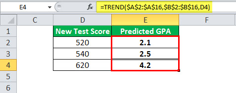
So, using the TREND function in Excel above, we predicted the three Y values for the new test scores.
Example #2 – Predicting the Sales Growth
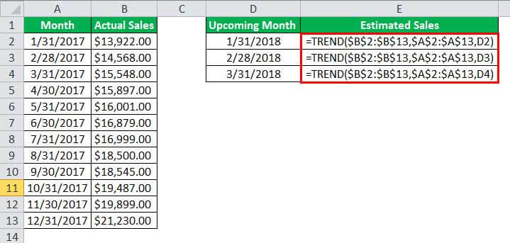
So in this example, we have existing sales data of a company for 2017 that increases linearly from Jan 2017 to Dec 2017. So, we need to figure out the sales for the given upcoming months. That is, we need to predict the sales values based on the predictive values for last year's data.
The existing data contains the dates in column A and the sales revenue in column B. Next, we need to calculate the estimated sales value for the next 5 months. Historical data is given below:

We will use the TREND function in Excel to predict the sales for the upcoming months in the next year since the sales value is increasing linearly. Therefore, the given known values of Y are the sales revenue. The known values of X are the end dates of the month, and the new values of X are the dates for the next three months, 01/31/2018, 02/28/2018, and 03/31/2018. Finally, we need to compute the estimated sales values based on historical data in A1:B13.
The TREND formula in Excel will take the existing values of known X and Y. We will pass the new values of X to calculate the values of Y in cells E2, E3, and E4.
The TREND formula in Excel will be:
=TREND($B$2:$B$13,$A$2:$A$13,D2)
We fixed the range for known X and Y values and passed the new value of X as a reference value. Applying the same TREND formula in Excel to other cells we have,
Output:
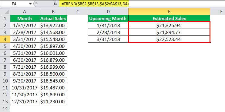
So, using the TREND function above, we have predicted the estimated sales values for the upcoming months in cells D2, D3, and D4.
Things to Remember
- The existing historical data that contains the known values of X and Y needs to be linear. For the given values of X, the value of Y should fit the linear curve y=m*x + c. Otherwise, the output or the predicted values may be inaccurate.
- The TREND function in Excel generates #VALUE! Error when the given known values of X or Y are non-numeric, or the value of new X is non-numeric, and when the const argument is not a Boolean value (that is TRUE or FALSE).
- The TREND function in Excel generates #REF! Because error known values of X and Y are of different lengths.
TREND Function in Excel Video
Recommended Articles
This article has been a guide to TREND Function in Excel. Here, we discuss the TREND formula in Excel and how to use the TREND function in Excel, along with Excel examples and downloadable Excel templates. You may also look at these useful functions in Excel: –
- Inserting Date in Excel In excel, every valid date will be stored as a form of the number. One important thing to be aware in excel is that we have got a cut-off date which is "31-Dec-1899". Every date we insert in excel will be counted from "01-Jan-1900 (including this date)" and will be stored as a number. read more
- Formula of Sales Revenue
- Top Best Differences Regression vs. ANOVA Both the Regression and ANOVA are the statistical models which are used in order to predict the continuous outcome but in case of the regression, continuous outcome is predicted on basis of the one or more than one continuous predictor variables whereas in case of ANOVA continuous outcome is predicted on basis of the one or more than one categorical predictor variables. read more
- Convert Excel Columns to Rows There are two ways to convert columns to rows: 1) using the Excel Ribbon Method. 2) The Mouse Method. read more
- VLOOKUP Wildcard Wildcard Characters are used with the VLOOKUP function to avail the lookup value by only using the partial match. It helps make VLOOKUP more powerful & avoids the #N/A Error. read more
Source: https://www.wallstreetmojo.com/trend-function-in-excel/
0 Response to "Can I Get Excel to Recognize a Trend and Continue It"
Post a Comment